Askaryan Frequency Content

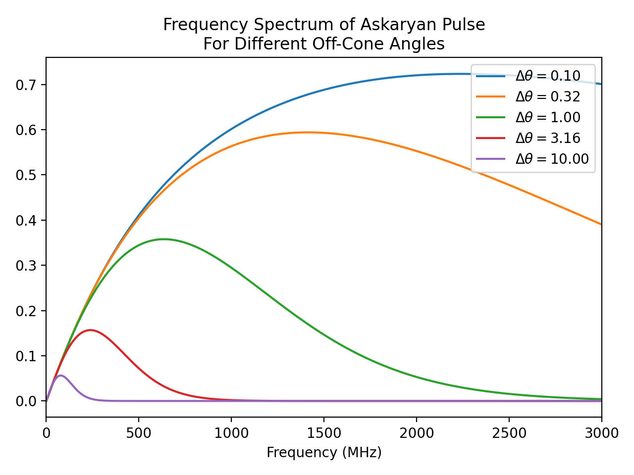
In this example we explore how the frequency spectrum of an Askaryan pulse changes as a function of the off-cone angle (i.e. the angular distance between the Cherenkov angle and the observation angle). This code can be run from the frequency_content.py script in the examples directory.

import numpy as np
import matplotlib.pyplot as plt
import pyrex

# First, set up a neutrino source and find the index of refraction at its depth.
# Then use that index of refraction to calculate the Cherenkov angle.
source = pyrex.Particle("nu_e", vertex=(0, 0, -1000), direction=(0, 0, -1),
                        energy=1e8)
n = pyrex.ice.index(source.vertex[2])
ch_angle = np.arccos(1/n)

# Now, for a range of dthetas, generate an Askaryan pulse dtheta away from the
# Chereknov angle and plot its frequency spectrum.
for dtheta in np.radians(np.logspace(-1, 1, 5)):
    n_pts = 10001
    pulse = pyrex.AskaryanSignal(times=np.linspace(-20e-9, 80e-9, n_pts),
                                 particle=source,
                                 viewing_angle=ch_angle+dtheta,
                                 viewing_distance=1000)
    plt.plot(pulse.frequencies[:int(n_pts/2)] * 1e-6, # Convert from Hz to MHz
             np.abs(pulse.spectrum)[:int(n_pts/2)],
             label=f"$\\Delta\\theta = {np.degrees(dtheta):.2f}$")
plt.legend(loc='upper right')
plt.title("Frequency Spectrum of Askaryan Pulse\n"+
          "For Different Off-Cone Angles")
plt.xlabel("Frequency (MHz)")
plt.xlim(0, 3000)
plt.tight_layout()
plt.show()

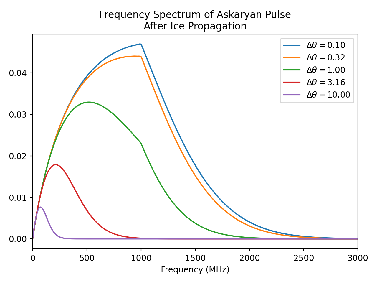
# Actually, we probably really want to see the frequency content after the
# signal has propagated through the ice a bit. So first set up the ray tracer
# from our neutrino source to some other point where our antenna might be
# (and make sure a path between those two points exists).
rt = pyrex.RayTracer(from_point=source.vertex, to_point=(500, 0, -100))
if not rt.exists:
    raise ValueError("Path to antenna doesn't exist!")

# Finally, plot the signal spectrum as it appears at the antenna position by
# propagating it along the (first solution) path.
path = rt.solutions[0]
for dtheta in np.radians(np.logspace(-1, 1, 5)):
    n_pts = 2048
    pulse = pyrex.AskaryanSignal(times=np.linspace(-20e-9, 80e-9, n_pts),
                                 particle=source,
                                 viewing_angle=ch_angle+dtheta,
                                 viewing_distance=path.path_length)
    pulse = path.propagate(pulse)
    plt.plot(pulse.frequencies[:int(n_pts/2)] * 1e-6, # Convert from Hz to MHz
             np.abs(pulse.spectrum)[:int(n_pts/2)],
             label=f"$\\Delta\\theta = {np.degrees(dtheta):.2f}$")
plt.legend(loc='upper right')
plt.title("Frequency Spectrum of Askaryan Pulse\n"+
          "After Ice Propagation")
plt.xlabel("Frequency (MHz)")
plt.xlim(0, 3000)
plt.tight_layout()
plt.show()

# You may notice the sharp cutoff in the frequency spectrum above 1 GHz.
# This is due to the ice model, which defines the attenuation length in a
# piecewise manner for frequencies above or below 1 GHz.