How to Use PyREx
This section describes in detail how to use a majority of the functions and classes included in the base PyREx package, along with short example code segments. The code in each section is designed to run sequentially, and the code examples all assume these imports:
import numpy as np
import matplotlib.pyplot as plt
import scipy.fft
import scipy.signal
import pyrex
All of the following examples can also be found (and easily run) in the Code Examples python notebook found in the examples directory.
Working with Signal Objects
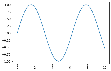
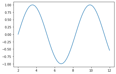
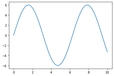
The base Signal class consists of an array of times and an array of corresponding signal values, and is instantiated with these two arrays. The times array is assumed to be in units of seconds, but there are no general units for the values array. It is worth noting that the Signal object stores shallow copies of the passed arrays, so changing the original arrays will not affect the Signal object.
time_array = np.linspace(0, 10)
value_array = np.sin(time_array)
my_signal = pyrex.Signal(times=time_array, values=value_array)
Plotting the Signal object is as simple as plotting the times vs the values:
plt.plot(my_signal.times, my_signal.values)
plt.show()
While there are no specified units for Signal.values, there is the option to specify the value_type of the values. This is done using the Signal.Type enum. By default, a Signal object has value_type=Type.unknown. However, if the signal represents a voltage, electric field, or power; value_type can be set to Signal.Type.voltage, Signal.Type.field, or Signal.Type.power respectively:
my_voltage_signal = pyrex.Signal(times=time_array, values=value_array,
                                 value_type=pyrex.Signal.Type.voltage)
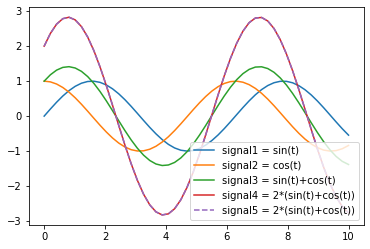
Signal objects can be added as long as they have the same time array and value_type. Signal objects can also be multiplied by numeric types, which will multiply the values attribute of the signal.
time_array = np.linspace(0, 10)
values1 = np.sin(time_array)
values2 = np.cos(time_array)
signal1 = pyrex.Signal(time_array, values1)
plt.plot(signal1.times, signal1.values,
         label="signal1 = sin(t)")
signal2 = pyrex.Signal(time_array, values2)
plt.plot(signal2.times, signal2.values,
         label="signal2 = cos(t)")
signal3 = signal1 + signal2
plt.plot(signal3.times, signal3.values,
         label="signal3 = sin(t)+cos(t)")
signal4 = 2 * signal3
plt.plot(signal4.times, signal4.values,
         label="signal4 = 2*(sin(t)+cos(t))")
all_signals = [signal1, signal2, signal3]
signal5 = sum(all_signals)
plt.plot(signal5.times, signal5.values, '--',
         label="signal5 = 2*(sin(t)+cos(t))")
plt.legend()
plt.show()
The Signal class provides many convenience attributes for dealing with signals:
my_signal.dt == my_signal.times[1] - my_signal.times[0]
my_signal.spectrum == scipy.fft.fft(my_signal.values)
my_signal.frequencies == scipy.fft.fftfreq(n=len(my_signal.values),
                                           d=my_signal.dt)
my_signal.envelope == np.abs(scipy.signal.hilbert(my_signal.values))
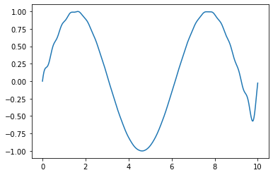
The Signal class also provides methods for manipulating the signal. The Signal.resample() method will resample the times and values arrays to the given number of points (with the same endpoints). This method operates “in-place” on the signal, but we can use the Signal.copy() method to make a duplicate object first so that further uses of the original signal object are unaffected:
signal_copy = my_signal.copy()
signal_copy.resample(1001)
len(signal_copy.times) == len(signal_copy.values) == 1001
signal_copy.times[0] == 0
signal_copy.times[-1] == 10
plt.plot(signal_copy.times, signal_copy.values)
plt.show()
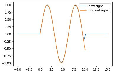
The Signal.with_times() method will interpolate/extrapolate the signal’s values onto a new times array:
new_times = np.linspace(-5, 15)
new_signal = my_signal.with_times(new_times)
plt.plot(new_signal.times, new_signal.values, label="new signal")
plt.plot(my_signal.times, my_signal.values, label="original signal")
plt.legend()
plt.show()
The Signal.shift() method will shift the signal in time by a specified value (in seconds):
my_signal.shift(2)
plt.plot(my_signal.times, my_signal.values)
plt.show()
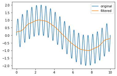
The Signal.filter_frequencies() method will apply a frequency-domain filter to the values array based on the frequency response function provided. In cases where the filter is designed for only positive frequencies (as below) the filtered frequency may exhibit strange behavior, including potentially having an imaginary part. To resolve that issue, pass force_real=True to the Signal.filter_frequencies() method, which will extrapolate the given filter to negative frequencies and ensure a real-valued filtered signal.
def lowpass_filter(frequency):
    if frequency < 1:
        return 1
    else:
        return 0

time_array = np.linspace(0, 10, 1001)
value_array = np.sin(0.1*2*np.pi*time_array) + np.sin(2*2*np.pi*time_array)
my_signal = pyrex.Signal(times=time_array, values=value_array)

plt.plot(my_signal.times, my_signal.values, label="original")
my_signal.filter_frequencies(lowpass_filter, force_real=True)
plt.plot(my_signal.times, my_signal.values, label="filtered")
plt.legend()
plt.show()
A number of classes which inherit from the Signal class are included in PyREx: EmptySignal, FunctionSignal, AskaryanSignal, and ThermalNoise.
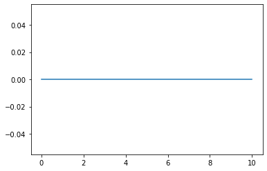
EmptySignal is simply a signal whose values are all zero:
time_array = np.linspace(0,10)
empty = pyrex.EmptySignal(times=time_array)
plt.plot(empty.times, empty.values)
plt.show()
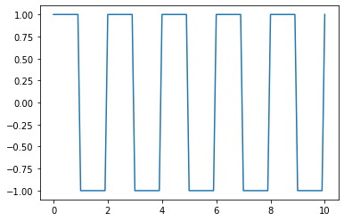
FunctionSignal takes a function of time and creates a signal based on that function:
time_array = np.linspace(0, 10, num=101)
def square_wave(time):
    if int(time)%2==0:
        return 1
    else:
        return -1
square_signal = pyrex.FunctionSignal(times=time_array, function=square_wave)
plt.plot(square_signal.times, square_signal.values)
plt.show()
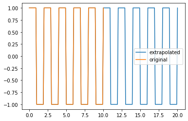
Additionally, FunctionSignal leverages its knowledge of the function to more accurately interpolate and extrapolate values for the Signal.with_times() method:
new_times = np.linspace(0, 20, num=201)
long_square_signal = square_signal.with_times(new_times)
plt.plot(long_square_signal.times, long_square_signal.values, label="extrapolated")
plt.plot(square_signal.times, square_signal.values, label="original")
plt.legend()
plt.show()
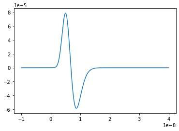
AskaryanSignal produces an Askaryan pulse (in V/m) on a time array resulting from a given neutrino observed at a given angle from the shower axis and at a given distance from the shower vertex. For more about using the Particle class, see Particle Generation.
time_array = np.linspace(-10e-9, 40e-9, 1001)
neutrino_energy = 1e8 # GeV
neutrino = pyrex.Particle("nu_e", vertex=(0, 0, -1000), direction=(0, 0, -1),
                          energy=neutrino_energy)
neutrino.interaction.em_frac = 1
neutrino.interaction.had_frac = 0
observation_angle = 65 * np.pi/180 # radians
observation_distance = 2000 # meters
askaryan = pyrex.AskaryanSignal(times=time_array, particle=neutrino,
                                viewing_angle=observation_angle,
                                viewing_distance=observation_distance)
print(askaryan.value_type)
plt.plot(askaryan.times, askaryan.values)
plt.show()
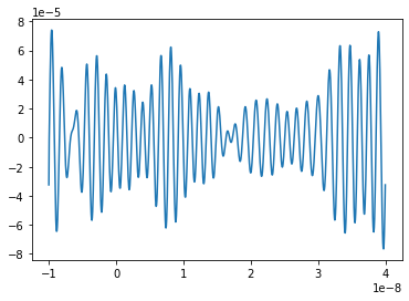
ThermalNoise produces Rayleigh-distributed noise (in V) at a given temperature and resistance, within a given frequency range:
time_array = np.linspace(-10e-9, 40e-9, 1001)
noise_temp = 300 # K
system_resistance = 1000 # ohm
frequency_range = (550e6, 750e6) # Hz
noise = pyrex.ThermalNoise(times=time_array, temperature=noise_temp,
                           resistance=system_resistance,
                           f_band=frequency_range)
print(noise.value_type)
plt.plot(noise.times, noise.values)
plt.show()
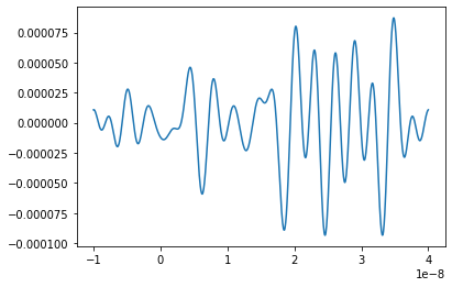
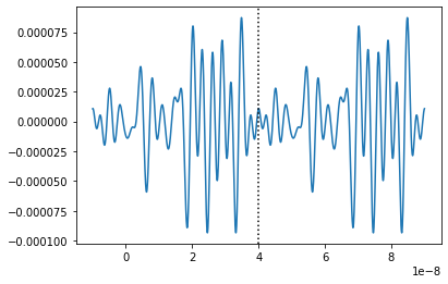
Note that since ThermalNoise inherits from FunctionSignal, it can be extrapolated nicely to new times. It may be highly periodic outside of its original time range however, but this can be tuned using the uniqueness_factor parameter.
short_noise = pyrex.ThermalNoise(times=time_array, temperature=noise_temp,
                                 resistance=system_resistance,
                                 f_band=(100e6, 400e6))
long_noise = short_noise.with_times(np.linspace(-10e-9, 90e-9, 2001))

plt.plot(short_noise.times, short_noise.values)
plt.show()
plt.plot(long_noise.times, long_noise.values)
plt.axvline(40e-9, ls=':', c='k')
plt.show()
Antenna Class and Subclasses
The base Antenna class provided by PyREx is designed to be subclassed in order to match various antenna models. At its core, an Antenna object is initialized with a position and a number of optional parameters, including a temperature, resistance, and frequency range (for noise calculations) and a boolean dictating whether or not noise should be added to the antenna’s signals.
# Please note that some values are unrealistic for demonstration purposes
position = (0, 0, -100) # m
temperature = 300 # K
resistance = 1e17 # ohm
frequency_range = (0, 5) # Hz
basic_antenna = pyrex.Antenna(position=position, temperature=temperature,
                              resistance=resistance,
                              freq_range=frequency_range)
noiseless_antenna = pyrex.Antenna(position=position, noisy=False)
The basic useful properties of an Antenna object are is_hit and waveforms. The is_hit property specifies whether or not the antenna has been triggered by an event. waveforms is a list of all the waveforms which have triggered the antenna. The antenna also defines a signals attribute, which is a list of all signals the antenna has received (without noise), and all_waveforms which is a list of all waveforms (signal plus noise) the antenna has received including those which didn’t trigger. Finally, the antenna has an is_hit_mc property which is similar to is_hit, but does not count triggers where noise alone would have triggered the antenna.
basic_antenna.is_hit == False
basic_antenna.waveforms == []
The Antenna class contains two attributes and three methods which represent characteristics of the antenna as they relate to signal processing. The attributes are efficiency and antenna_factor, and the methods are Antenna.frequency_response(), Antenna.directional_gain(), and Antenna.polarization_gain(). The attributes are to be set and the methods overwritten in order to customize the way the antenna responds to incoming signals. efficiency is simply a scalar which multiplies the signal the antenna receives (default value is 1). antenna_factor is a factor used in converting received electric fields into voltages (antenna_factor = E / V; default value is 1). Antenna.frequency_response() takes a frequency or list of frequencies (in Hz) and returns the frequency response of the antenna at each frequency given (default always returns 1). Antenna.directional_gain() takes angles theta and phi in the antenna’s coordinates and returns the antenna’s gain for a signal coming from that direction (default always returns 1). Antenna.directional_gain() is dependent on the antenna’s orientation, which is defined by its z_axis and x_axis attributes. To change the antenna’s orientation, use the Antenna.set_orientation() method which takes z_axis and x_axis arguments. Finally, Antenna.polarization_gain() takes a polarization vector and returns the antenna’s gain for a signal with that polarization (default always returns 1).
basic_antenna.efficiency == 1
basic_antenna.antenna_factor == 1
freqs = [1, 2, 3, 4, 5]
basic_antenna.frequency_response(freqs) == [1, 1, 1, 1, 1]
basic_antenna.directional_gain(theta=np.pi/2, phi=0) == 1
basic_antenna.polarization_gain([0,0,1]) == 1
The Antenna class defines an Antenna.trigger() method which is also expected to be overwritten. Antenna.trigger() takes a Signal object as an argument and returns a boolean of whether or not the antenna would trigger on that signal (default always returns True).
basic_antenna.trigger(pyrex.Signal([0],[0])) == True
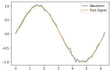
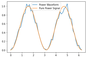
The Antenna class also defines an Antenna.receive() method which takes a Signal object and processes the signal according to the antenna’s attributes (efficiency, antenna_factor, response, directional_gain, and polarization_gain as described above). To use the Antenna.receive() method, simply pass it the Signal object the antenna sees, and the Antenna class will handle the rest. You can also optionally specify the direction of travel of the signal (used in the Antenna.directional_gain() calculation) and the polarization direction of the signal (used in the Antenna.polarization_gain() calculation). If either of these is unspecified, the corresponding gain will simply be set to 1.
def limited_sin(times, min_time, max_time):
values = np.zeros(len(times))
in_range = (times>=min_time) & (times<max_time)
values[in_range] = np.sin(times[in_range])
return values
incoming_signal_1 = pyrex.FunctionSignal(np.linspace(0,2*np.pi), lambda t: limited_sin(t,0,2*np.pi),
value_type=pyrex.Signal.Type.voltage)
incoming_signal_2 = pyrex.FunctionSignal(np.linspace(4*np.pi,6*np.pi), lambda t: limited_sin(t,4*np.pi,6*np.pi),
value_type=pyrex.Signal.Type.voltage)
basic_antenna.receive(incoming_signal_1)
basic_antenna.receive(incoming_signal_2, direction=[0,0,1], polarization=[1,0,0])
basic_antenna.is_hit == True
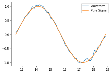
for waveform, pure_signal in zip(basic_antenna.waveforms, basic_antenna.signals):
plt.figure()
plt.plot(waveform.times, waveform.values, label="Waveform")
plt.plot(pure_signal.times, pure_signal.values, label="Pure Signal")
plt.legend()
plt.show()
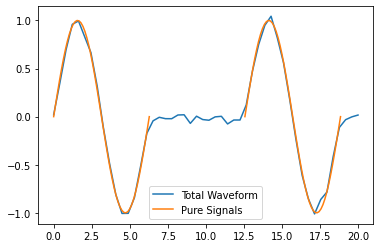
Beyond Antenna.waveforms, the Antenna object also provides methods for checking the waveform and trigger status for arbitrary times: Antenna.full_waveform() and Antenna.is_hit_during(). Both of these methods take a time array as an argument and return either the waveform Signal object for those times or whether said waveform triggered the antenna, respectively.
total_waveform = basic_antenna.full_waveform(np.linspace(0,20))
plt.plot(total_waveform.times, total_waveform.values, label="Total Waveform")
plt.plot(incoming_signal_1.times, incoming_signal_1.values, label="Pure Signals")
plt.plot(incoming_signal_2.times, incoming_signal_2.values, color="C1")
plt.legend()
plt.show()

basic_antenna.is_hit_during(np.linspace(0,6)) == True
Finally, the Antenna class defines an Antenna.clear() method which will reset the antenna to a state of having received no signals:
basic_antenna.clear()
basic_antenna.is_hit == False
len(basic_antenna.waveforms) == 0
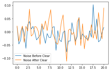
The Antenna.clear() method can also optionally reset the source of noise waveforms by passing reset_noise=True so that if the same signals are given after the antenna is cleared, the noise waveforms will be different:
noise_before = basic_antenna.make_noise(np.linspace(0, 20))
plt.plot(noise_before.times, noise_before.values, label="Noise Before Clear")
basic_antenna.clear(reset_noise=True)
noise_after = basic_antenna.make_noise(np.linspace(0, 20))
plt.plot(noise_after.times, noise_after.values, label="Noise After Clear")
plt.legend()
plt.show()
To create a custom antenna, simply inherit from the Antenna class:
class NoiselessThresholdAntenna(pyrex.Antenna):
    def __init__(self, position, threshold):
        super().__init__(position=position, noisy=False)
        self.threshold = threshold

    def trigger(self, signal):
        if max(np.abs(signal.values)) > self.threshold:
            return True
        else:
            return False
Our custom NoiselessThresholdAntenna should only trigger when the amplitude of a signal exceeds its threshold value:
my_antenna = NoiselessThresholdAntenna(position=(0, 0, 0), threshold=2)

incoming_signal = pyrex.FunctionSignal(np.linspace(0,10), np.sin,
                                       value_type=pyrex.Signal.Type.voltage)
my_antenna.receive(incoming_signal)
my_antenna.is_hit == False
len(my_antenna.waveforms) == 0
len(my_antenna.all_waveforms) == 1

incoming_signal = pyrex.Signal(incoming_signal.times,
                               5*incoming_signal.values,
                               incoming_signal.value_type)
my_antenna.receive(incoming_signal)
my_antenna.is_hit == True
len(my_antenna.waveforms) == 1
len(my_antenna.all_waveforms) == 2

for wave in my_antenna.waveforms:
    plt.figure()
    plt.plot(wave.times, wave.values)
    plt.show()
For more on customizing PyREx, see the Custom Sub-Package section.
PyREx also defines DipoleAntenna, a subclass of Antenna which provides a basic threshold trigger, a basic bandpass filter frequency response, a sine-function directional gain, and a typical dot-product polarization effect. A DipoleAntenna object can be created as follows:
antenna_identifier = "antenna 1"
position = (0, 0, -100)
center_frequency = 250e6 # Hz
bandwidth = 300e6 # Hz
temperature = 300 # K
resistance = 100 # ohm
antenna_length = 3e8/center_frequency/2 # m
polarization_direction = (0, 0, 1)
trigger_threshold = 1e-5 # V
dipole = pyrex.DipoleAntenna(name=antenna_identifier,position=position,
                             center_frequency=center_frequency,
                             bandwidth=bandwidth,
                             temperature=temperature, resistance=resistance,
                             effective_height=antenna_length,
                             orientation=polarization_direction,
                             trigger_threshold=trigger_threshold)
AntennaSystem and Detector Classes
The AntennaSystem class is designed to bridge the gap between the basic antenna classes and realistic antenna systems that include front-end processing of the antenna’s signals. It is designed to be subclassed, but by default it takes as an argument the Antenna class or subclass it is extending, or an object of that class. It provides an interface nearly identical to that of the Antenna class, but where an AntennaSystem.front_end() method (which by default does nothing) is applied to the extended antenna’s signals.
To extend an Antenna class or subclass into a full antenna system, inherit from the AntennaSystem class and define the AntennaSystem.front_end() method. If the front end of the antenna system requires some time to equilibrate to noise signals, that can be specified in the AntennaSystem.lead_in_time attribute, adding that amount of time before any waveforms to be processed. A different trigger also optionally can be defined for the antenna system (by default it uses the antenna’s trigger):
class PowerAntennaSystem(pyrex.AntennaSystem):
    """Antenna system whose signals and waveforms are powers instead of
    voltages."""
    def __init__(self, position, temperature, resistance, frequency_range):
        super().__init__(pyrex.Antenna)
        # The setup_antenna method simply passes all arguments on to the
        # antenna class passed to super.__init__() and stores the resulting
        # antenna to self.antenna
        self.setup_antenna(position=position, temperature=temperature,
                           resistance=resistance,
                           freq_range=frequency_range)

    def front_end(self, signal):
        return pyrex.Signal(signal.times, signal.values**2,
                            value_type=pyrex.Signal.Type.power)
Objects of this class can then, for the most part, be interacted with as though they were regular antenna objects:
position = (0, 0, -100) # m
temperature = 300 # K
resistance = 1e17 # ohm
frequency_range = (0, 5) # Hz
basic_antenna_system = PowerAntennaSystem(position=position,
temperature=temperature,
resistance=resistance,
frequency_range=frequency_range)
basic_antenna_system.trigger(pyrex.Signal([0],[0])) == True
def limited_sin(times, min_time, max_time):
values = np.zeros(len(times))
in_range = (times>=min_time) & (times<max_time)
values[in_range] = np.sin(times[in_range])
return values
incoming_signal_1 = pyrex.FunctionSignal(np.linspace(0,2*np.pi), lambda t: limited_sin(t,0,2*np.pi),
value_type=pyrex.Signal.Type.voltage)
incoming_signal_2 = pyrex.FunctionSignal(np.linspace(4*np.pi,6*np.pi), lambda t: limited_sin(t,4*np.pi,6*np.pi),
value_type=pyrex.Signal.Type.voltage)
basic_antenna_system.receive(incoming_signal_1)
basic_antenna_system.receive(incoming_signal_2, direction=[0,0,1],
polarization=[1,0,0])
basic_antenna_system.is_hit == True
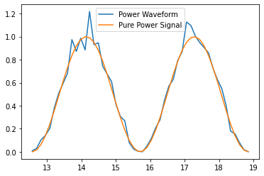
for waveform, pure_signal in zip(basic_antenna_system.waveforms,
basic_antenna_system.signals):
plt.figure()
plt.plot(waveform.times, waveform.values, label="Waveform")
plt.plot(pure_signal.times, pure_signal.values, label="Pure Signal")
plt.legend()
plt.show()
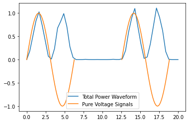
total_waveform = basic_antenna_system.full_waveform(np.linspace(0,20))
plt.plot(total_waveform.times, total_waveform.values, label="Total Waveform")
plt.plot(incoming_signal_1.times, incoming_signal_1.values, label="Pure Signals")
plt.plot(incoming_signal_2.times, incoming_signal_2.values, color="C1")
plt.legend()
plt.show()
basic_antenna_system.is_hit_during(np.linspace(0,6)) == True
basic_antenna_system.clear()
basic_antenna_system.is_hit == False
len(basic_antenna_system.waveforms) == 0
The Detector class is another convenience class meant to be subclassed. It is useful for automatically generating many antennas (as would be used in a detector). Subclasses must define a Detector.set_positions() method to assign vector positions to the antenna_positions attribute. By default Detector.set_positions() will raise a NotImplementedError. Additionally subclasses may extend the default Detector.build_antennas() method which by default simply builds antennas of a passed antenna class using any keyword arguments passed to the method. In addition to simply generating many antennas at desired positions, another convenience of the Detector class is that once the Detector.build_antennas() method is run, it can be iterated directly as though the object were a list of the antennas it generated. And finally, the Detector.triggered() method will check whether any of the antennas have been triggered, and can be overridden in subclasses to define a more complicated detector trigger. An example of subclassing the Detector class is shown below:
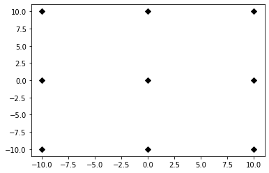
class AntennaGrid(pyrex.Detector):
    """A detector composed of a plane of antennas in a rectangular grid layout
    some distance below the ice."""
    def set_positions(self, number, separation=10, depth=-50):
        self.antenna_positions = []
        n_x = int(np.sqrt(number))
        n_y = int(number/n_x)
        dx = separation
        dy = separation
        for i in range(n_x):
            x = -dx*n_x/2 + dx/2 + dx*i
            for j in range(n_y):
                y = -dy*n_y/2 + dy/2 + dy*j
                self.antenna_positions.append((x, y, depth))

grid_detector = AntennaGrid(9)

# Build the antennas
temperature = 300 # K
resistance = 1e17 # ohm
frequency_range = (0, 5) # Hz
grid_detector.build_antennas(pyrex.Antenna, temperature=temperature,
                             resistance=resistance,
                             freq_range=frequency_range)

plt.figure(figsize=(6,6))
for antenna in grid_detector:
    x = antenna.position[0]
    y = antenna.position[1]
    plt.plot(x, y, "kD")
plt.ylim(plt.xlim())
plt.show()
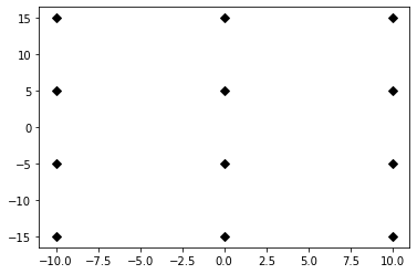
Due to the parallels between Antenna and AntennaSystem, an antenna system may also be used in the custom detector class. Note however, that the antenna positions must be accessed as antenna.antenna.position since we didn’t define a position attribute for the PowerAntennaSystem:
grid_detector = AntennaGrid(12)

# Build the antennas
temperature = 300 # K
resistance = 1e17 # ohm
frequency_range = (0, 5) # Hz
grid_detector.build_antennas(PowerAntennaSystem, temperature=temperature,
                            resistance=resistance,
                            frequency_range=frequency_range)

for antenna in grid_detector:
    x = antenna.antenna.position[0]
    y = antenna.antenna.position[1]
    plt.plot(x, y, "kD")
plt.show()
For convenience, objects derived from the Detector class can be added into a CombinedDetector object, which behaves similarly. The CombinedDetector.build_antennas() method should work seamlessly if the sub-detectors have the same build_antennas() method, otherwise it will do its best to dispatch keyword arguments between the sub-detectors. Similarly the CombinedDetector.triggered() method will return True if either sub-detector was triggered, with arguments to the method dispatched to the proper sub-triggers.
Ice and Earth Models
PyREx provides an ice model object ice, which is an instance of whichever ice model class is preferred (currently pyrex.ice_model.AntarcticIce). The ice object provides a number of (hopefully self-explanatory) methods for calculating characteristics of the ice at different depths and frequencies as below:
depth = -1000 # m
pyrex.ice.temperature(depth)
pyrex.ice.index(depth)
pyrex.ice.gradient(depth)
frequency = 1e8 # Hz
pyrex.ice.attenuation_length(depth, frequency)
PyREx also provides an Earth model object earth, which is similarly an instance of whichever Earth model class is preferred (currently pyrex.earth_model.PREM). This model provides two methods: density() and slant_depth(). density() calculates the density in grams per cubic centimeter of the Earth at a given radius, and slant_depth() calculates the material thickness in grams per square centimeter of a chord cutting through the Earth in a given direction, starting from a given point:
radius = 6360000 # m
pyrex.earth.density(radius)
angle = 60 * np.pi/180 # radians
direction = (np.sin(angle), 0, -np.cos(angle))
endpoint = (0, 0, -1000) # m
pyrex.earth.slant_depth(endpoint, direction)
Ray Tracing
PyREx provides ray tracing in the RayTracer and RayTracePath classes. RayTracer takes a launch point and receiving point as arguments (and optionally an ice model and z-step), and will solve for the paths between the points (as RayTracePath objects).
start = (0, 0, -250) # m
finish = (750, 0, -100) # m
my_ray_tracer = pyrex.RayTracer(from_point=start, to_point=finish)
The two most useful properties of RayTracer are exists and solutions. The exists property is a boolean value of whether or not path solutions exist between the launch and receiving points. solutions is the list of (zero or two) RayTracePath objects which exist between the launch and receiving points. There are many other properties available in RayTracer, outlined in the PyREx API section, which are mostly used internally and maybe not interesting otherwise.
my_ray_tracer.exists
my_ray_tracer.solutions
The RayTracePath class contains the attributes of the paths between points. The most useful properties of RayTracePath are tof, path_length, emitted_direction, and received_direction. These properties provide the time of flight, path length, and direction of rays at the launch and receiving points respectively.
my_path = my_ray_tracer.solutions[0]
my_path.tof
my_path.path_length
my_path.emitted_direction
my_path.received_direction
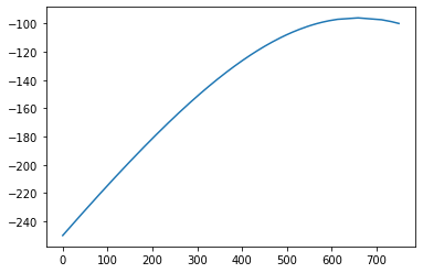
RayTracePath also provides a RayTracePath.attenuation() method which gives the attenuation of the signal at a given frequency (or frequencies), and a RayTracePath.coordinates property which gives the x, y, and z coordinates of the path (useful mostly for plotting, and not guaranteed to be accurate enough for other purposes).
frequency = 100e6 # Hz
my_path.attenuation(frequency)
my_path.attenuation(np.linspace(1e8, 1e9, 11))
plt.plot(my_path.coordinates[0], my_path.coordinates[2])
plt.show()
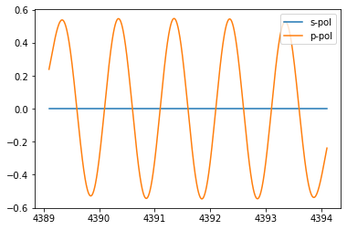
Finally, RayTracePath.propagate() propagates a Signal object from the launch point to the receiving point of the path by applying the frequency-dependent attenuation from RayTracePath.attenuation(), and shifting the signal times by RayTracePath.tof. Note that it does not apply a 1/R factor to the signal amplitude based on the path length. If needed, this effect should be added in manually. RayTracePath.propagate() returns the Signal objects and polarization vectors of the s-polarized and p-polarized portions of the signal.
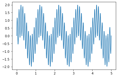
time_array = np.linspace(0, 5e-9, 1001)
launch_signal = (
    pyrex.FunctionSignal(time_array, lambda t: np.sin(1e9*2*np.pi*t))
    + pyrex.FunctionSignal(time_array, lambda t: np.sin(1e10*2*np.pi*t))
)
plt.plot(launch_signal.times*1e9, launch_signal.values)
plt.show()
# Polarize perpendicular to the path in the x-z plane
launch_pol = np.cross(my_path.emitted_direction, (0, 1, 0))
print(launch_pol)

rec_signals, rec_pols = my_path.propagate(launch_signal, polarization=launch_pol)
plt.plot(rec_signals[0].times*1e9, rec_signals[0].values, label="s-pol signal")
plt.plot(rec_signals[1].times*1e9, rec_signals[1].values, label="p-pol signal")
plt.legend()
plt.show()
print(rec_pols)
Particle Generation
PyREx includes the Particle class as a container for information about neutrinos which are generated to produce Askaryan pulses. A Particle contains an id, a vertex, a direction, an energy, an interaction, and a weight:
particle_type = pyrex.Particle.Type.electron_neutrino
initial_position = (0,0,0) # m
direction_vector = (0,0,-1)
particle_energy = 1e8 # GeV
particle = pyrex.Particle(particle_id=particle_type, vertex=initial_position,
                          direction=direction_vector, energy=particle_energy)
The interaction attribute is an instance of an Interaction class (NeutrinoInteraction by default) which is a model for how the neutrino interacts in the ice. It has a kind denoting whether the interaction will be charged-current or neutral-current, an inelasticity, em_frac and had_frac describing the resulting particle shower(s), and cross_section and interaction_length in the ice at the energy of the parent Particle object:
type(particle.interaction)
particle.interaction.kind
particle.interaction.inelasticity
particle.interaction.em_frac
particle.interaction.had_frac
particle.interaction.cross_section
particle.interaction.interaction_length
PyREx also includes a number of classes for generating random neutrinos in various ice volumes. The CylindricalGenerator and RectangularGenerator classes generate neutrinos uniformly in cylindrical or rectangular volumes respectively. These generator classes take as arguments the necessary dimensions and an energy (which can be a scalar value or a function returning scalar values). Additional arguments include whether to reject events shadowed by the Earth, as well as a desired flavor ratio:
volume_radius = 1000 # m
volume_depth = 500 # m
flavor_ratio = (1, 1, 1) # even distribution of neutrino flavors
source = 'astrophysical' # could also be cosmogenic, changes neutrino:antineutrino ratios
my_generator = pyrex.CylindricalGenerator(dr=volume_radius,
                                          dz=volume_depth,
                                          energy=particle_energy,
                                          shadow=False,
                                          flavor_ratio=flavor_ratio,
                                          source=source)
my_generator.create_event()
The create_event() method of the generator returns an Event object, which contains a tree of Particle objects representing the event. Currently this tree will only contain a single neutrino, but could be expanded in the future in order to describe more exotic events. The neutrino is available as the only element in the list Event.roots. It can also be accessed by iterating the Event object.
Lastly, PyREx includes ListGenerator and FileGenerator classes which can be used to reproduce pre-generated events from either a list or from simulation output files, respectively. For example, to continuously re-throw our Particle object from above:
repetitive_generator = pyrex.ListGenerator([pyrex.Event(particle)])
repetitive_generator.create_event()
repetitive_generator.create_event()
Full Simulation
PyREx provides the EventKernel class to control a basic simulation including the creation of neutrinos and their respective signals, the propagation of their pulses to the antennas, and the triggering of the antennas. The EventKernel is designed to be modular and can use a specific ice model, ray tracer, output file writer, and signal times array as specified in optional arguments, along with some basic parameters used to speed up the simulation (the defaults are explicitly specified below).
The EventKernel.event() method handles the full simulation of a single event: generating a random neutrino event with a corresponding Askaryan signal, propagating the signal to each antenna in the detector, and processing the response of the antennas to the incoming signal(s). The method returns the Event object simulated and optionally may return whether the detector was triggered by the event.
particle_generator = pyrex.CylindricalGenerator(dr=1000, dz=1000, energy=1e8)
detector = []
for i, z in enumerate([-100, -150, -200, -250]):
detector.append(
pyrex.DipoleAntenna(name="antenna_"+str(i), position=(0, 0, z),
center_frequency=250e6, bandwidth=300e6,
temperature=300, resistance=0, effective_height=0.6,
trigger_threshold=1e-4, noisy=False)
)
kernel = pyrex.EventKernel(generator=particle_generator,
antennas=detector,
ice_model=pyrex.ice,
ray_tracer=pyrex.RayTracer,
signal_times=np.linspace(-50e-9, 50e-9, 2000,
endpoint=False),
event_writer=None, triggers=None,
offcone_max=40, weight_min=None,
attenuation_interpolation=0.1)
triggered = False
while not triggered:
for antenna in detector:
antenna.clear()
event = kernel.event()
for antenna in detector:
if antenna.is_hit:
triggered = True
break
particle = event.roots[0]
print("Particle type: ", particle.id)
print("Shower vertex: ", particle.vertex)
print("Shower axis: ", particle.direction)
print("Particle energy: ", particle.energy)
print("Interaction type:", particle.interaction.kind)
print("Electromagnetic shower fraction:", particle.interaction.em_frac)
print("Hadronic shower fraction: ", particle.interaction.had_frac)
print("Event weight:", particle.weight)
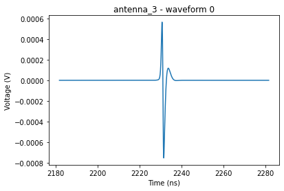
for antenna in detector:
for i, wave in enumerate(antenna.waveforms):
plt.plot(wave.times * 1e9, wave.values)
plt.xlabel("Time (ns)")
plt.ylabel("Voltage (V)")
plt.title(antenna.name + " - waveform "+str(i))

Data File I/O
The File class controls the reading and writing of data files for simulation. At the most basic it takes a filename and mode in which to open the file, and if the file type is supported the object will be the appropriate file handler. Like python’s open() function, the File class works as a context manager and should preferably be used in with statements. Currently the only data file type supported by PyREx is HDF5. Depending on whether an HDF5 file is being read or written there are additional keyword arguments that may be provided to File. HDF5 files support the following modes: ‘r’ for read-only, ‘w’ for write (overwrites existing file), ‘a’/’r+’ for append (doesn’t overwrite existing file), and ‘x’ for write (fails if file exists already).
If writing an HDF5 file, the optional arguments specify which event data to write. The available write options are write_particles, write_triggers, write_antenna_triggers, write_rays, write_noise, and write_waveforms. Most of these are self-explanatory, but write_antenna_triggers will write triggering information for each antenna in the detector and write_noise will write the frequency data required to replicate noise waveforms. The last optional argument is require_trigger which specifies which data should only be written when the detector is triggered. If a boolean value, requires trigger or not for all data with the exception of particle and trigger data, which is always written. If a list of strings, the listed data will require triggers and any other data will always be written.
The most straightforward way to write data files is to pass a File object to the EventKernel object handling the simulation. In such a case, a global trigger condition should be passed to the EventKernel as well, either as a function which acts on a detector object, or as the “global” key in a dictionary of functions representing various trigger conditions:
particle_generator = pyrex.CylindricalGenerator(dr=1000, dz=1000, energy=1e8)
detector = []
for i, z in enumerate([-100, -150, -200, -250]):
    detector.append(
        pyrex.DipoleAntenna(name="antenna_"+str(i), position=(0, 0, z),
                            center_frequency=250e6, bandwidth=300e6,
                            temperature=300, resistance=0, effective_height=0.6,
                            trigger_threshold=1e-8, noisy=False)
    )

def global_trigger_condition(det):
    for ant in det:
        if ant.is_hit:
            return True
    return False

def even_antenna_trigger(det):
    for i, ant in enumerate(det):
        if i%2==0 and ant.is_hit:
            return True
    return False

trigger_conditions = {
    "global": global_trigger_condition,
    "evens": even_antenna_trigger,
    "ant1": lambda det: det[1].is_hit
}

with pyrex.File('my_data_file.h5', 'w') as f:
    kernel = pyrex.EventKernel(generator=particle_generator,
                               antennas=detector,
                               event_writer=f,
                               triggers=trigger_conditions)

    for _ in range(10):
        for antenna in detector:
            antenna.clear()
        event, triggered = kernel.event()
        print(triggered)
If you want to manually write the data file, then the File.set_detector() and File.add() methods are necessary. File.set_detector() associates the given antennas with the file object (and writes their data) and File.add() adds the data from the given event to the file. Here we also manually open and close the file object with File.open() and File.close(), and add some metadata to the file with File.add_file_metadata():
f = pyrex.File('my_data_file_2.h5', 'w')
f.open()

f.add_file_metadata({"write_style": "manual", "number_of_events": 10})

f.set_detector(detector)

kernel = pyrex.EventKernel(generator=particle_generator,
                           antennas=detector)

for _ in range(10):
    for antenna in detector:
        antenna.clear()
    event = kernel.event()
    triggered = False
    for antenna in detector:
        if antenna.is_hit:
            triggered = True
            break
    f.add(event, triggered=triggered)

f.close()
The File objects also support writing miscellaneous analysis data to the file. File.create_analysis_dataset() creates and returns a basic HDF5 dataset. File.create_analysis_metadataset() creates a joined set of tables for string and float data, which can be written to with File.add_analysis_metadata(). And finally, File.add_analysis_indices() allows for linking event indices to specific rows of analysis data.
with pyrex.File('my_data_file.h5', 'a') as f:
    f.create_analysis_metadataset("effective_volume")
    gen_vol = (np.pi*1000**2)*1000
    # Just set an arbitrary number of triggers for now. We'll get into reading
    # files in the examples below.
    n_triggers = 5
    data = {
        "generation_volume": gen_vol,
        "veff": n_triggers/10*gen_vol,
        "error": np.sqrt(n_triggers)/10*gen_vol,
        "unit": "m^3"
    }
    f.add_analysis_metadata("effective_volume", data)

    other = f.create_analysis_dataset("meaningless_data",
                                      data=np.ones((20, 5)))
    other.attrs['rows_per_event'] = 2
    for i in range(10):
        f.add_analysis_indices("meaningless_data", global_index=i,
                               start_index=2*i, length=2)
If reading an HDF5 file, the slice_range argument specifies the size of event slices to load into memory at once when iterating over events. In general, increasing the slice_range will improve the speed of iteration at the cost of greater memory consumption. By default, the whole file is read at once.
with pyrex.File('my_data_file.h5', 'r', slice_range=100) as f:
    pass
When reading HDF5 files, there are a number of methods and attributes available to access the data. With the File object alone, File.file_metadata contains a dictionary of the file’s metadata and File.antenna_info contains a list of dictionaries with data for each antenna in the detector the file was run with. If waveform data is available, File.get_waveforms() can be used to get all waveforms in the file or a specific subset based on event_id, antenna_id, and waveform_type arguments. Finally, direct access to the contents of the HDF5 file is supported through either the proper paths or nicknames.
with pyrex.File('my_data_file.h5', 'r') as f:
    print(f.file_metadata)
    print(f.antenna_info[0])

    # No waveform data was stored above, so these will fail if run
    # All waveforms:
    # wfs = f.get_waveforms()
    # Waveforms from event 0
    # wfs = f.get_waveforms(event_id=0)
    # Waveforms in antenna 1 from all events
    # wfs = f.get_waveforms(antenna_id=1)
    # Direct waveform in antenna 4 from event 5
    # wf = f.get_waveforms(event_id=5, antenna_id=4, waveform_type=0)

    # Using full file path
    triggers = f['data/triggers']
    # Using dataset nickname
    particle_string_metadata = f['particles_meta_str']
    # Using analysis dataset nickname
    other = f['meaningless_data']
HDF5 files opened in read-only mode can also be iterated over, which allows access to the data for each event in turn. When iterating, the event objects have the following methods for accessing data. get_particle_info() and get_rays_info() return a list of dictionaries or attribute values for the event’s particles or rays, respectively. The is_neutrino, is_nubar, and flavor attributes also contain the associated basic information about the base particle of the event. get_waveforms() returns the waveforms for the event, or a specific subset based on antenna_id and waveform_type (as above). The triggered attribute contains whether the event triggered the detector and the get_triggered_components() method returns a list of the trigger conditions of the detector which were met (as specified when writing the file). And finally, if noise data is recorded for the event it is contained in the noise_bases attribute. Iteration of the HDF5 files supports slicing as long as the step size is positive-valued, and individual events can also be reached by indexing the File object.
with pyrex.File('my_data_file.h5', 'r') as f:
    for event in f:
        print(event.is_neutrino, event.is_nubar, event.flavor)
        print(event.triggered, event.get_triggered_components())
    print()

    for event in f[2:6:2]:
        print(event.get_particle_info('particle_name'),
              event.get_particle_info('vertex'))
        print(np.degrees(event.get_rays_info('receiving_angle')))
    print()

    print(f[4].get_rays_info('tof'))

    # No waveform data was stored above, so this will fail if run
    # wfs = f[4].get_waveforms(antenna_id=2)
More Examples
For more code examples, see the Example Code section and the python notebooks and scripts in the examples directory.