Examine a Single Event

In this example we will generate a single event with a given vertex, direction, and energy, and then we’ll examine the event by plotting the waveforms. This is typically useful for auditing events from a larger simulation. This code can be run from the examine_event.py script in the examples directory.

import numpy as np
import matplotlib.pyplot as plt
import pyrex
import pyrex.custom.ara as ara

# First let's rebuild our detector that was used in the simulation.
det = ara.RegularStation(x=0, y=0, antennas_per_string=4,
                         antenna_separation=[2, 18, 2])
det.build_antennas(power_threshold=-6.15)

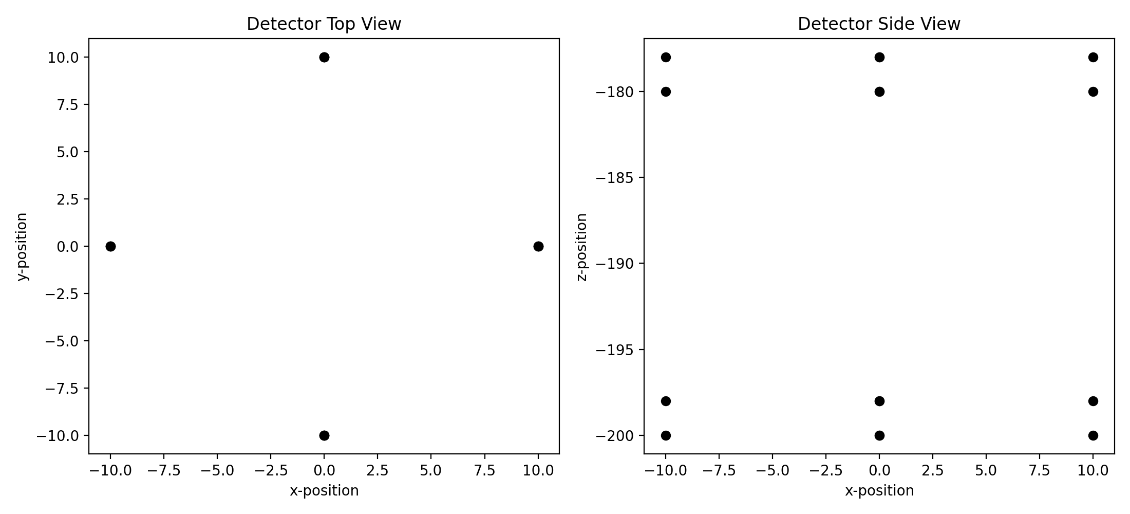
# Then let's plot a couple views of it just to be sure everything looks right.
fig, ax = plt.subplots(1, 2, figsize=(11, 5))
ax[0].scatter([ant.position[0] for ant in det],
              [ant.position[1] for ant in det],
              c='k')
ax[0].set_title("Detector Top View")
ax[0].set_xlabel("x-position")
ax[0].set_ylabel("y-position")
ax[1].scatter([ant.position[0] for ant in det],
              [ant.position[2] for ant in det],
              c='k')
ax[1].set_title("Detector Side View")
ax[1].set_xlabel("x-position")
ax[1].set_ylabel("z-position")
plt.tight_layout()
plt.show()

# Now set up a particle generator that will just throw the one event we're
# interested in, and create an event kernel with our detector and our generator.
p = pyrex.Particle(particle_id=pyrex.Particle.Type.electron_neutrino,
                   vertex=[1002.65674195, -421.95118348, -486.0953201],
                   direction=[-0.90615395, -0.41800062, -0.06450191],
                   energy=3e9)
p.interaction.kind = p.interaction.Type.neutral_current
p.interaction.em_frac = 0
p.interaction.had_frac = 1
gen = pyrex.ListGenerator(pyrex.Event(p))
kern = pyrex.EventKernel(antennas=det, generator=gen)

# Then make sure our detector is cleared out and throw the event!
# reset_noise will make sure we get new noise waveforms every time.
det.clear(reset_noise=True)
kern.event()

# Now let's take a look at the waveforms of the event. Since each event has a
# first and second ray, plot their waveforms side-by-side for each antenna.
for i, ant in enumerate(det):
    fig, ax = plt.subplots(1, 2, figsize=(12, 3))
    for j, wave in enumerate(ant.all_waveforms):
        ax[j].plot(wave.times*1e9, wave.values)
        ax[j].set_xlabel("Time (ns)")
        ax[j].set_ylabel("Amplitude (V)")
        ax[j].set_title("First Ray" if j%2==0 else "Second Ray")
    fig.suptitle("String "+str(int(i/4))+" "+ant.name)
    plt.tight_layout()
    plt.show()

# From the plots it looks like the first ray is the one that triggered the
# detector. Let's calculate a signal-to-noise ratio of the first-ray waveform
# for each antenna.
print("Signal-to-noise ratios:")
for i, ant in enumerate(det):
    wave = ant.all_waveforms[0]
    signal_pp = np.max(wave.values) - np.min(wave.values)
    noise = ant.front_end(ant.antenna.make_noise(wave.times))
    noise_rms = np.sqrt(np.mean(noise.values**2))
    print("  String "+str(int(i/4))+" "+ant.name+":", signal_pp/(2*noise_rms))

# Let's also take a look at the trigger condition, which passes the waveform
# through a tunnel diode. Again we can plot the tunnel diode's integrated
# waveform for each ray side-by-side. The red lines indicate the trigger level.
# If the integrated waveform goes beyond those lines the antenna is triggered.
for i, ant in enumerate(det):
    fig, ax = plt.subplots(1, 2, figsize=(12, 3))
    for j, wave in enumerate(ant.all_waveforms):
        triggered = ant.trigger(wave)
        trigger_wave = ant.tunnel_diode(wave)
        # The first time ant.trigger is run for an antenna, the power mean and
        # rms are calculated which will determine the trigger condition.
        low_trigger = (ant._power_mean -
                       ant._power_std*np.abs(ant.power_threshold))
        high_trigger = (ant._power_mean +
                        ant._power_std*np.abs(ant.power_threshold))
        ax[j].plot(trigger_wave.times*1e9, trigger_wave.values)
        ax[j].axhline(low_trigger, color='r')
        ax[j].axhline(high_trigger, color='r')
        ax[j].set_title("Triggered" if triggered else "Missed")
        ax[j].set_xlabel("Time (ns)")
        ax[j].set_ylabel("Integrated Power (V^2)")
    fig.suptitle("String "+str(int(i/4))+" "+ant.name)
    plt.tight_layout()
    plt.show()

# Finally, let's look at the relative trigger times to make sure they look
# reasonable. We could get the true relative trigger times from the waveforms
# by just taking the differences of their first times, but instead let's
# pretend we're doing an analysis and just use the times of the maxima.
trig_times = []
for ant in det:
    wave = ant.all_waveforms[0]
    trig_times.append(wave.times[np.argmax(np.abs(wave.values))])

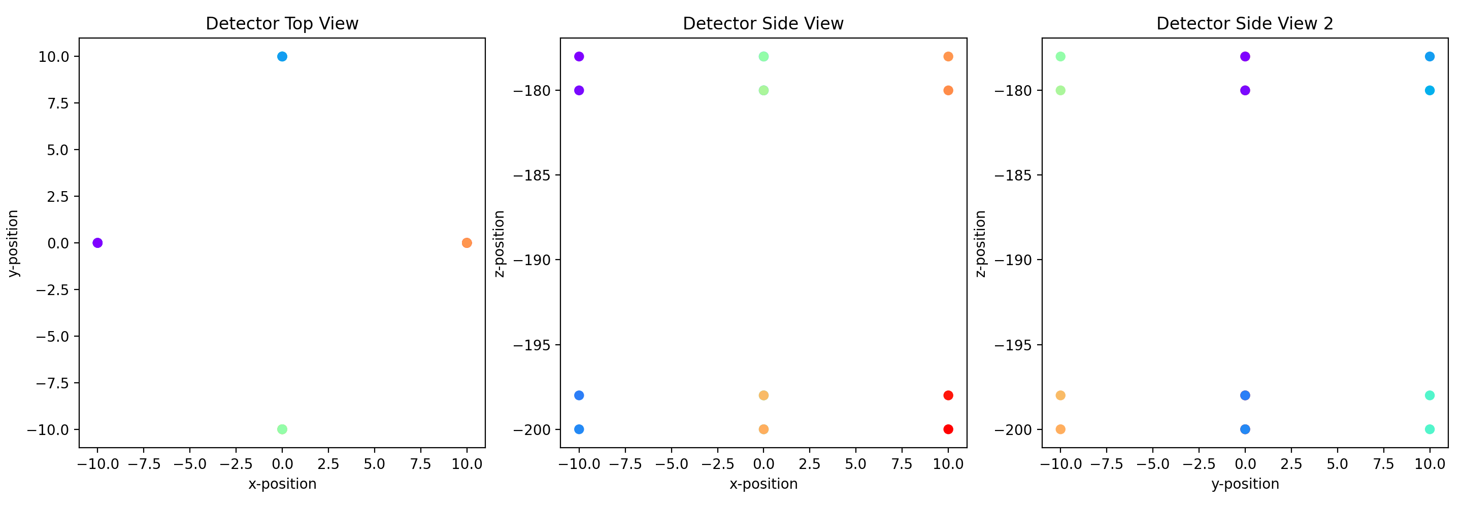
# Then we can plot the progression of the event by coloring the antennas where
# red is the earliest time and blue/purple is the latest time.
fig, ax = plt.subplots(1, 3, figsize=(16, 5))
ax[0].scatter([ant.position[0] for ant in det],
              [ant.position[1] for ant in det],
              c=trig_times, cmap='rainbow_r')
ax[0].set_title("Detector Top View")
ax[0].set_xlabel("x-position")
ax[0].set_ylabel("y-position")
ax[1].scatter([ant.position[0] for ant in det],
              [ant.position[2] for ant in det],
              c=trig_times, cmap='rainbow_r')
ax[1].set_title("Detector Side View")
ax[1].set_xlabel("x-position")
ax[1].set_ylabel("z-position")
ax[2].scatter([ant.position[1] for ant in det],
              [ant.position[2] for ant in det],
              c=trig_times, cmap='rainbow_r')
ax[2].set_title("Detector Side View 2")
ax[2].set_xlabel("y-position")
ax[2].set_ylabel("z-position")
plt.tight_layout()
plt.show()